Trypanosoma phyloseq

Last updated: 2021-07-03

Checks: 7 0

Knit directory: wildlife-haemoprotozoa/

This reproducible R Markdown analysis was created with workflowr (version 1.6.2). The Checks tab describes the reproducibility checks that were applied when the results were created. The Past versions tab lists the development history.

R Markdown file: up-to-date

Great! Since the R Markdown file has been committed to the Git repository, you know the exact version of the code that produced these results.

Environment: empty

Great job! The global environment was empty. Objects defined in the global environment can affect the analysis in your R Markdown file in unknown ways. For reproduciblity it’s best to always run the code in an empty environment.

Seed: set.seed(20210212)

The command set.seed(20210212) was run prior to running the code in the R Markdown file. Setting a seed ensures that any results that rely on randomness, e.g. subsampling or permutations, are reproducible.

Session information: recorded

Great job! Recording the operating system, R version, and package versions is critical for reproducibility.

Cache: none

Nice! There were no cached chunks for this analysis, so you can be confident that you successfully produced the results during this run.

File paths: relative

Great job! Using relative paths to the files within your workflowr project makes it easier to run your code on other machines.

Repository version: 63bd5ef

Great! You are using Git for version control. Tracking code development and connecting the code version to the results is critical for reproducibility.

The results in this page were generated with repository version 63bd5ef. See the Past versions tab to see a history of the changes made to the R Markdown and HTML files.

Note that you need to be careful to ensure that all relevant files for the analysis have been committed to Git prior to generating the results (you can use wflow_publish or wflow_git_commit). workflowr only checks the R Markdown file, but you know if there are other scripts or data files that it depends on. Below is the status of the Git repository when the results were generated:


Ignored files:
    Ignored:    .DS_Store
    Ignored:    .Rhistory
    Ignored:    .Rproj.user/
    Ignored:    analysis/.DS_Store
    Ignored:    analysis/.Rhistory
    Ignored:    analysis/_footer.html
    Ignored:    data/.DS_Store
    Ignored:    output/.DS_Store

Untracked files:
    Untracked:  ENA_submission/
    Untracked:  NCBI_submission/
    Untracked:  Rplot02.pdf
    Untracked:  data/NGS_18S_kinet/
    Untracked:  data/Sanger-piroplasm/
    Untracked:  data/haemoprotozoa.csv
    Untracked:  data/haemoprotozoa.xlsx
    Untracked:  data/tryp-phyloseq/count_data_QC.xlsx
    Untracked:  data/tryp-phyloseq/count_data_raw.csv
    Untracked:  data/tryp-phyloseq/sampledata.xlsx
    Untracked:  melt.csv
    Untracked:  melt.xlsx
    Untracked:  microscopy/
    Untracked:  output/plots/

Unstaged changes:
    Modified:   README.md
    Modified:   code/usearchv11_18S_Kineto.sh

Note that any generated files, e.g. HTML, png, CSS, etc., are not included in this status report because it is ok for generated content to have uncommitted changes.

These are the previous versions of the repository in which changes were made to the R Markdown (analysis/tryp-02-phyloseq.Rmd) and HTML (docs/tryp-02-phyloseq.html) files. If you’ve configured a remote Git repository (see ?wflow_git_remote), click on the hyperlinks in the table below to view the files as they were in that past version.

File	Version	Author	Date	Message
Rmd	63bd5ef	siobhon-egan	2021-07-03	Formatting and setup updates
html	4608186	siobhon-egan	2021-07-02	footer
html	483a08b	siobhon-egan	2021-07-02	Build site.
Rmd	b1f7e30	siobhon-egan	2021-07-02	include main figs and tables
html	a36fbcb	siobhon-egan	2021-07-02	Build site.
Rmd	8e3850e	siobhon-egan	2021-07-02	Major update

Visualization and analysis of trypanosome NGS data data.

Note this was run using R version 4.0.3 and RStudo version 1.4. See R info for full details of R session.

0. Load libraries

Install libraries if required

Only need to run this code once.

if (!requireNamespace("BiocManager", quietly = TRUE))
    install.packages("BiocManager")
# phyloseq
source('http://bioconductor.org/biocLite.R')
biocLite('phyloseq')
#tidyverse
install. packages("tidyverse")
#ampvis2
install.packages("remotes")
remotes::install_github("MadsAlbertsen/ampvis2")
#ampvis2extras
install.packages("BiocManager")
BiocManager::install("kasperskytte/ampvis2extras")
#ggpubr
install.packages("ggpubr")
#agricolae
install.packages("agricolae")
install.packages("remotes")
remotes::install_github("DanielSprockett/reltools")
devtools::install_github('jsilve24/philr')
#decontam
BiocManager::install("decontam")
library(decontam)
if (!requireNamespace("BiocManager", quietly = TRUE))
install.packages("BiocManager")
BiocManager::install("Biostrings")

Load libraries

pkgs <- c("qiime2R", "phyloseq", "tidyverse", "ampvis2",
          "ampvis2extras", "ggpubr", "agricolae", "plotly",
          "viridis", "cowplot", "MicrobeR", "microbiome",
          "reshape", "decontam", "data.table", "ape",
          "DESeq2", "vegan", "microbiomeutilities", "knitr",
          "tibble", "dplyr","patchwork", "Biostrings")

lapply(pkgs, require, character.only = TRUE)

theme_set(theme_bw())

1. Import data

Generate phyloseq object from spreadsheets.

Import ASV/OTU count data

count_data <- read_csv("data/tryp-phyloseq/count_data_cleaned.csv")
# use first column as label for rows
count_data_lab = column_to_rownames(count_data, var = "#Zotu ID")
# Make matrix
otumat <- as.matrix(count_data_lab)

Import taxonomy data

taxonomy <- read_csv("data/tryp-phyloseq/taxonomy.csv", 
    col_types = cols(Accession_description = col_skip(), 
        `Accession no.` = col_skip(), evalue = col_skip(), 
        `per. Ident` = col_skip(), taxid = col_skip()))
# use first column as label for rows
taxonomy_lab = column_to_rownames(taxonomy, var = "#Zotu ID")
taxmat <- as.matrix(taxonomy_lab)

Check the class of the otumat and taxmat objects, they MUST be in matrix format. Then we can great a phyloseq object called physeq from the otu and taxonomy tables and check the sample names.

class(otumat)
class(taxmat)
OTU = otu_table(otumat, taxa_are_rows = TRUE)
TAX = tax_table(taxmat)
physeq = phyloseq(OTU, TAX)
physeq
sample_names(physeq)

Add metadata and sequence data

Add sequences to phyloseq object

# read sequence file
rep.seqs <- Biostrings::readDNAStringSet("data/tryp-phyloseq/unoise_zotus.fasta", format = "fasta")

Add metadata, importing gDNAID as factor to be able to merge later on

metadata <- read_csv("data/tryp-phyloseq/sampledata.csv")
metadata_lab = column_to_rownames(metadata, var = "SampleID")
sampledata = sample_data(data.frame(metadata_lab))
sampledata

Create final phyloseq object

Now you can merge your data to create a final phyloseq object

ps_raw_tryp = merge_phyloseq(physeq, sampledata, rep.seqs)

Preliminary subset

Remove samples with NA values or not part of final data set,

ps_raw_tryp <- subset_samples(ps_raw_tryp, !SampleType=="SampleEcol")
ps_samp_tryp <- subset_samples(ps_raw_tryp, SampleType=="Sample")

Save/load `.RData`

Save R data for phyloseq object - saving “raw data” which inc controls (ps_raw_tryp) and “sample only data” (ps_samp_tryp)

save(ps_raw_tryp, file = "data/Rdata/ps_raw_tryp.RData")
save(ps_samp_tryp, file = "data/Rdata/ps_samp_tryp.RData")

To load raw and sample data quickly from .RData format.

load("data/Rdata/ps_raw_tryp.RData")
load("data/Rdata/ps_samp_tryp.RData")

An easy way to view the tables is using Nice Tables

Nice.Table(ps_samp_tryp@sam_data)

Nice.Table(ps_samp_tryp@tax_table)

2. QC plots

R package decontam to assess contaminating OTUs, tutorial.

The CRAN version only works on R version <4. To install for R versions >4 install from bioconductor using the following

Make plot of library size of Samples vs Controls

df <- as.data.frame(sample_data(ps_raw_tryp)) # Put sample_data into a ggplot-friendly data.frame
df$LibrarySize <- sample_sums(ps_raw_tryp)
df <- df[order(df$LibrarySize),]
df$Index <- seq(nrow(df))
libQC <- ggplot(data=df, aes(x=Index, y=LibrarySize, color=SampleType)) + geom_point() + theme_bw() + scale_colour_brewer(palette = "Set1")
libQC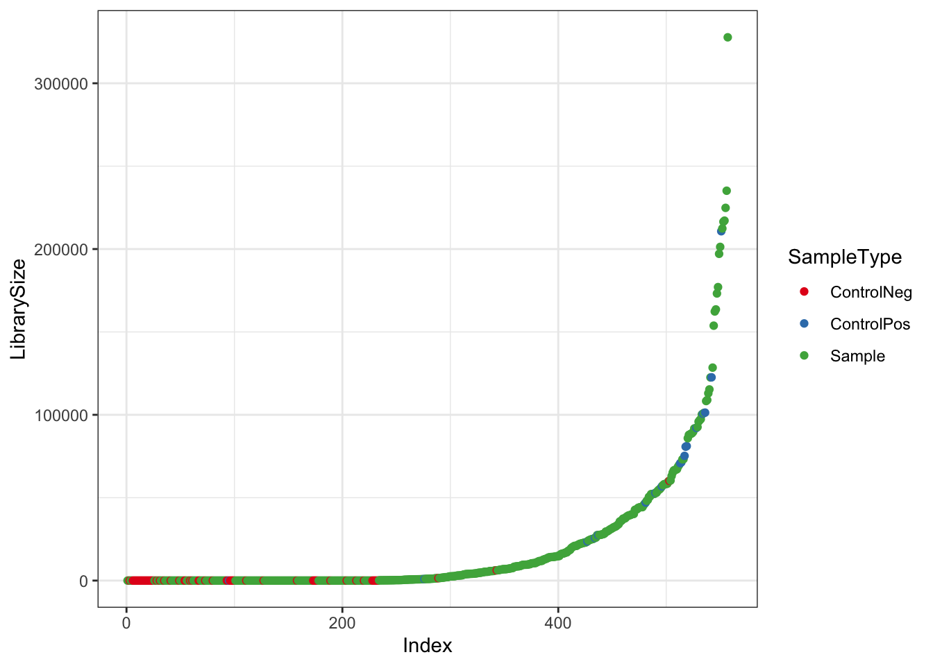

Version	Author	Date
483a08b	siobhon-egan	2021-07-02

#ggsave("libQC.pdf", plot = libQC, path = "output/plots/trypNGS", width = 15, height = 10, units = "cm")

Make html plot with plotly

libQCplotly <- ggplotly(libQC)
libQCplotly

#htmlwidgets::saveWidget(libQCplotly, "output/plots/libQCplotly.html")

Make distribution plot of reads using microbiomeutilities

distrib <- plot_read_distribution(ps_raw_tryp, groups = "SampleCategory", 
                            plot.type = "density") + xlab("Reads per sample") + ylab("Density")

[1] "Done plotting"

distrib <- distrib + geom_density(alpha = 0.5, fill = "grey") + theme(axis.text.x = element_text(angle = 45, size=10, vjust = 1))
distrib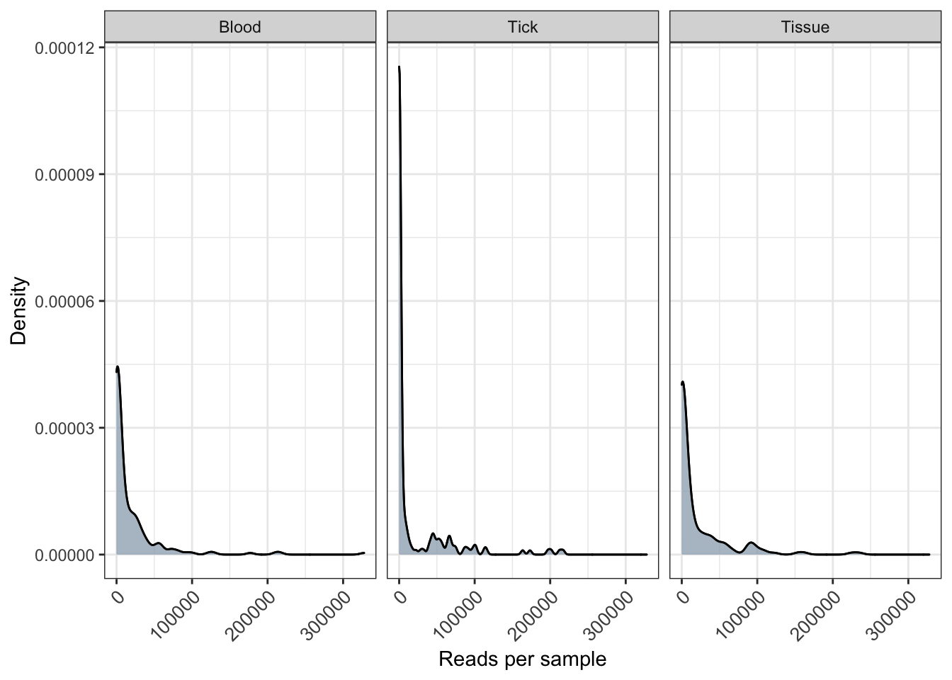

Version	Author	Date
483a08b	siobhon-egan	2021-07-02

#ggsave("distrib.pdf", plot = distrib, path = "output/plots/trypNGS", width = 15, height = 10, units = "cm")

Merge the two above plots into one figure.

QC <- ggarrange(libQC, distrib,
                    labels = c("A", "B"),
                    ncol = 1, nrow = 2)
#ggsave("QC.pdf", plot = QC, path = "output/plots/trypNGS", width = 20, height = 20, units = "cm")

3. Subset and Filter

3.1. For phyloseq object

Subset phyloseq object based on sample types

# samples and positive controls
ps_tryp_sampcon = subset_samples(ps_raw_tryp, SampleType=="Sample" | SampleType=="ControlPos")
# Blood samples only
ps_tryp_bl = subset_samples(ps_samp_tryp, SampleCategory=="Blood")
# Tissue samples only
ps_tryp_tis = subset_samples(ps_samp_tryp, SampleCategory=="Tissue")
# Tick samples only
ps_tryp_tick = subset_samples(ps_samp_tryp, SampleCategory=="Tick")

Subset phyloseq object based on host species

# Black rat
ps_BR = subset_samples(ps_samp_tryp, species=="Black rat")
# Brush tail possum
ps_BTP = subset_samples(ps_samp_tryp, species=="Brush tail possum")
# Chuditch
ps_chud = subset_samples(ps_samp_tryp, species=="Chuditch")
# Long-nosed bandicoot
ps_LNB = subset_samples(ps_samp_tryp, species=="Long-nosed bandicoot")

3.2. For ampvis2 object

Make ampvis2 object for analysis

#require the devtools package to source gist
if(!require("devtools"))
  install.packages("devtools")
#source the phyloseq_to_ampvis2() function from the gist
devtools::source_gist("8d0ca4206a66be7ff6d76fc4ab8e66c6")

#convert
tryp_amp <- phyloseq_to_ampvis2(ps_samp_tryp)

#save ampvis2 RData obj
save(tryp_amp, file = "data/Rdata/tryp_amp.RData")

Load in saved ampvis2 obj

load("data/Rdata/tryp_amp.RData")

Subset ampvis2 object based on sample category

#remove controls
amp_samp <- amp_subset_samples(tryp_amp, 
                                 !SampleType %in% c("ControlPos"),
                                 RemoveAbsents = TRUE)

0 samples have been filtered.

#blood samples
amp_bl <- amp_subset_samples(amp_samp, 
                                 SampleCategory %in% c("Blood"),
                                 RemoveAbsents = TRUE)

316 samples and 410 OTUs have been filtered 
Before: 477 samples and 587 OTUs
After: 161 samples and 177 OTUs

#tissue samples
am_tis <- amp_subset_samples(amp_samp, 
                                 SampleCategory %in% c("Tissue"),
                                 RemoveAbsents = TRUE)

321 samples and 214 OTUs have been filtered 
Before: 477 samples and 587 OTUs
After: 156 samples and 373 OTUs

#tick samples
amp_tick <- amp_subset_samples(amp_samp, 
                                 SampleCategory %in% c("Tick"),
                                 RemoveAbsents = TRUE)

317 samples and 512 OTUs have been filtered 
Before: 477 samples and 587 OTUs
After: 160 samples and 75 OTUs

4. Heatmap

4.1. ampvis2

Make heat map using ampvis2.

First filter taxa

# order Trypanosomatida
tax_vector1 <- c(
  "Trypanosomatida"
)

amp_samp_otry <- amp_subset_taxa(amp_samp,
  tax_vector = tax_vector1)

Warning: One or more samples have 0 total reads

542 OTUs have been filtered 
Before: 587 OTUs
After: 45 OTUs

# Trypanosoma species of interest
tax_vector2 <- c(
  "Trypanosoma gilletti",
  "Trypanosoma sp. (cyclops-like)",
  "Trypanosoma vegrandis",
  "Trypanosoma noyesi",
  "Trypanosoma sp. (lewisi-like)",
  "Lotmaria passim"
)

amp_samp_targettryp <- amp_subset_taxa(amp_samp,
  tax_vector = tax_vector2)

Warning: One or more samples have 0 total reads

544 OTUs have been filtered 
Before: 587 OTUs
After: 43 OTUs

Relative abundance

Heatmap of subsetted data using relative abundance

# Relative abundance order level trypanosome subset obj
heatmap_rel1 <- amp_heatmap(amp_samp_otry,
            facet_by = "SampleCategory",
            group_by = "species",
            tax_aggregate = "Species",
            tax_show = 10,
            normalise = TRUE,
            plot_values = FALSE,
            plot_values_size = 3,
            round = 0, color_vector = c("white", "#e5ba52", "#ab7ca3", "#9d02d7", "#0030bf"), plot_colorscale = "log10")  +
  theme(axis.text.x = element_text(angle = 45, size=10, vjust = 1),
        axis.text.y = element_text(size=10),
        legend.position="right")

Warning: There are only 7 taxa, showing all

heatmap_rel1

Warning: Transformation introduced infinite values in discrete y-axis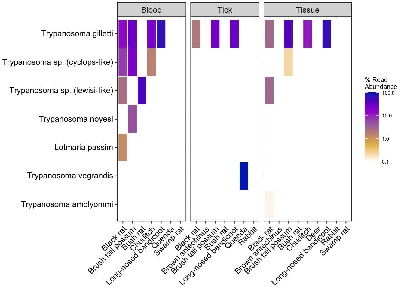

Version	Author	Date
483a08b	siobhon-egan	2021-07-02

# Relative abundance species level trypanosome subset obj
heatmap_rel2 <- amp_heatmap(amp_samp_targettryp,
            facet_by = "SampleCategory",
            group_by = "species",
            tax_aggregate = "Species",
            tax_show = 10,
            normalise = TRUE,
            plot_values = FALSE,
            plot_values_size = 3,
            round = 0, color_vector = c("white", "#e5ba52", "#ab7ca3", "#9d02d7", "#0030bf"), plot_colorscale = "log10")  +
  theme(axis.text.x = element_text(angle = 45, size=10, vjust = 1),
        axis.text.y = element_text(size=10),
        legend.position="right")

Warning: There are only 6 taxa, showing all

heatmap_rel2

Warning: Transformation introduced infinite values in discrete y-axis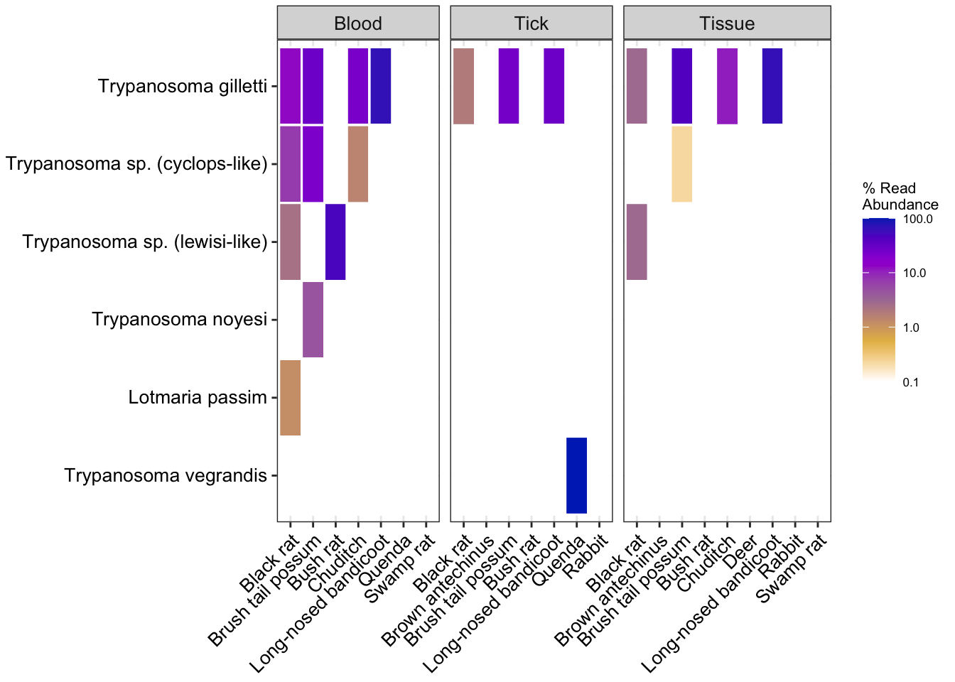

Version	Author	Date
483a08b	siobhon-egan	2021-07-02

Save PDF of plots

ggsave("heatmap_rel1.pdf", plot = heatmap_rel1, path = "output/plots/trypNGS", width = 25, height = 15, units = "cm")
ggsave("heatmap_rel2.pdf", plot = heatmap_rel2, path = "output/plots/trypNGS", width = 25, height = 15, units = "cm")

Count of sequences

heatmap_count <- amp_heatmap(amp_samp,
            facet_by = "SampleCategory",
            group_by = "species",
            tax_aggregate = "Family",
            tax_show = 40,
            normalise = FALSE,
            plot_values = FALSE,
            plot_values_size = 3,
            round = 0, color_vector = c("white", "#e5ba52", "#ab7ca3", "#9d02d7", "#0030bf"), plot_colorscale = "log10") + theme(axis.text.x = element_text(angle = 45, size=10, vjust = 1), axis.text.y = element_text(size=10), legend.position="right")
heatmap_count

4.2. microbiomeutilities

Heatmap using microbiomeutilities

Create a detailed heatmap using the micro utilities package.

Subset taxa of interest

ps_tryp_otry = subset_taxa(ps_samp_tryp, Order=="Trypanosomatida")
ps_tryp_subtry = subset_taxa(ps_samp_tryp, Species=="Trypanosoma gilletti" | Species=="Trypanosoma sp. (cyclops-like)" | Species =="Trypanosoma vegrandis" | Species=="Trypanosoma noyesi" | Species=="Trypanosoma sp. (lewisi-like)" | Species =="Lotmaria passim")

Creat plot

# create a gradient color palette for abundance
#grad_ab <- colorRampPalette(c("#faf3dd","#f7d486" ,"#5e6472"))
color_vector = colorRampPalette(c("#faf3dd", "#e5ba52", "#ab7ca3", "#9d02d7", "#0030bf"))
grad_ab_pal <- color_vector(10)

# create a color palette for varaibles of interest

meta_colors = list(c("Blood" = "#7a255d", "Tick" = "#9fd0cb", "Tissue" = "#7566ff"), 
                  c("Brush tail possum" = "#440154FF", "Black rat" = "#482878FF", "Swamp rat"="#3E4A89FF", "Long-nosed bandicoot" ="#31688EFF", "Bush rat"="#26828EFF", "Brown antechinus" = "#1F9E89FF", "Rabbit"="#35B779FF", "Chuditch"= "#6DCD59FF", "Quenda" = "#B4DE2CFF", "Deer" = "#FDE725FF" ))

# add labels for pheatmap to detect
names(meta_colors) <- c("SampleCategory", "species")

ph_heatmap <- plot_taxa_heatmap(ps_tryp_subtry,
                       subset.top = 50,
                       VariableA = c("SampleCategory","species"),
                       heatcolors = grad_ab_pal, #rev(brewer.pal(6, "RdPu")),
                       transformation = "log10",
                       cluster_rows = T,
                       cluster_cols = F,
                       show_colnames = F,
                       annotation_colors=meta_colors, fontsize = 8)

Top 50 OTUs selected

log10, if zeros in data then log10(1+x) will be used

First top taxa were selected and 
then abundances tranformed to log10(1+X)

Warning in transform(phyobj1, "log10"): OTU table contains zeroes. Using log10(1
+ x) transform.

ph_heatmap$plot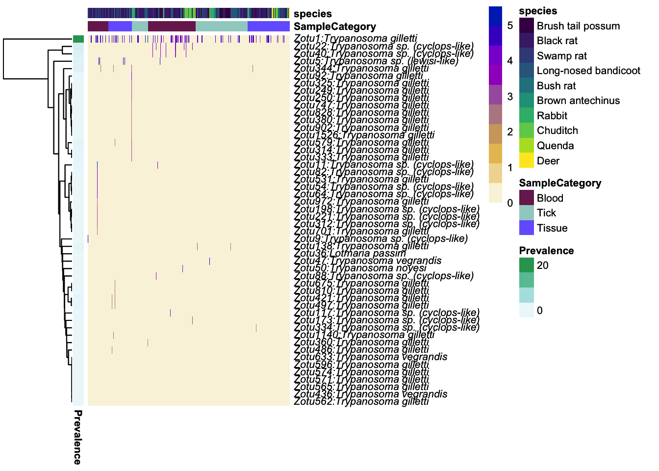

Version	Author	Date
483a08b	siobhon-egan	2021-07-02