Mapping
Last updated: 2022-03-07
Checks: 7 0
Knit directory: wildlife-ticks/
This reproducible R Markdown analysis was created with workflowr (version 1.7.0). The Checks tab describes the reproducibility checks that were applied when the results were created. The Past versions tab lists the development history.
Great! Since the R Markdown file has been committed to the Git repository, you know the exact version of the code that produced these results.
Great job! The global environment was empty. Objects defined in the global environment can affect the analysis in your R Markdown file in unknown ways. For reproduciblity it’s best to always run the code in an empty environment.
The command set.seed(20210211) was run prior to running the code in the R Markdown file. Setting a seed ensures that any results that rely on randomness, e.g. subsampling or permutations, are reproducible.
Great job! Recording the operating system, R version, and package versions is critical for reproducibility.
Nice! There were no cached chunks for this analysis, so you can be confident that you successfully produced the results during this run.
Great job! Using relative paths to the files within your workflowr project makes it easier to run your code on other machines.
Great! You are using Git for version control. Tracking code development and connecting the code version to the results is critical for reproducibility.
The results in this page were generated with repository version 7b4fd7e. See the Past versions tab to see a history of the changes made to the R Markdown and HTML files.
Note that you need to be careful to ensure that all relevant files for the analysis have been committed to Git prior to generating the results (you can use wflow_publish or wflow_git_commit). workflowr only checks the R Markdown file, but you know if there are other scripts or data files that it depends on. Below is the status of the Git repository when the results were generated:
Ignored files:
    Ignored:    .DS_Store
    Ignored:    .Rhistory
    Ignored:    .Rproj.user/
    Ignored:    analysis/.DS_Store
    Ignored:    analysis/_footer.html
    Ignored:    output/.DS_Store
    Ignored:    output/plots/.DS_Store

Untracked files:
    Untracked:  .Rprofile
    Untracked:  ENA_submission/
    Untracked:  NCBI_submission/
    Untracked:  analysis/images/
    Untracked:  data/
    Untracked:  experiments/
    Untracked:  flex.Rmd
    Untracked:  flex.html
    Untracked:  list.csv
    Untracked:  output/plots/allmap1.pdf
    Untracked:  output/plots/allmap2.pdf
    Untracked:  output/plots/allmapala1.pdf
    Untracked:  output/plots/allmapala2.pdf
    Untracked:  output/plots/combined-map5.pdf
    Untracked:  output/plots/combined-map6.pdf
    Untracked:  output/plots/combined-map7.pdf
    Untracked:  output/plots/combined-map8.pdf
    Untracked:  output/plots/map-ala.html
    Untracked:  output/plots/map-ala_files/
    Untracked:  output/plots/map-all-ala.html
    Untracked:  output/plots/map-all-ala_files/
    Untracked:  output/plots/map-all-curated.html
    Untracked:  output/plots/map-all-curated_files/
    Untracked:  output/plots/map-atrig-facet-edit.pdf
    Untracked:  output/plots/map-atrig-facet-edit.png
    Untracked:  output/plots/map-atrig-facet-edit.svg
    Untracked:  output/plots/map-atrig-subspecies1.pdf
    Untracked:  output/plots/map-atrig-subspecies2.pdf
    Untracked:  output/plots/map-atrig1.pdf
    Untracked:  output/plots/map-atrig2.pdf
    Untracked:  output/plots/map-ixhol1-edit.pdf
    Untracked:  output/plots/map-ixhol1-edit.png
    Untracked:  output/plots/map-ixhol1-edit.svg
    Untracked:  output/plots/map-ixtas1-edit.pdf
    Untracked:  output/plots/map-ixtas1-edit.png
    Untracked:  output/plots/map-ixtas1-edit.svg
    Untracked:  output/plots/maplegend-ala.pdf
    Untracked:  output/plots/maplegend-edit.pdf
    Untracked:  output/plots/maplegend-edit.png
    Untracked:  output/plots/maplegend-edit.svg
    Untracked:  output/plots/maplegend.pdf
    Untracked:  speciesNames.csv
    Untracked:  temp/

Unstaged changes:
    Modified:   README.md
    Modified:   analysis/_site.yml
    Deleted:    analysis/mapping.Rmd
    Deleted:    output/plots/combined-map.pdf
    Modified:   output/plots/combined-map1.pdf
    Modified:   output/plots/combined-map2.pdf
    Modified:   output/plots/combined-map3.pdf
    Modified:   output/plots/combined-map4.pdf
    Deleted:    output/plots/map-atrig-comb-nolegend.pdf
    Deleted:    output/plots/map-atrig-comb.pdf
    Modified:   output/plots/map-atrig-facet.pdf
    Deleted:    output/plots/map-atrig-simple1.pdf
    Deleted:    output/plots/map-atrig-simple2.pdf
    Modified:   output/plots/map-ixhol1.pdf
    Modified:   output/plots/map-ixhol2.pdf
    Modified:   output/plots/map-ixtas1.pdf
    Modified:   output/plots/map-ixtas2.pdf
Note that any generated files, e.g. HTML, png, CSS, etc., are not included in this status report because it is ok for generated content to have uncommitted changes.
These are the previous versions of the repository in which changes were made to the R Markdown (analysis/mapsFigures.Rmd) and HTML (docs/mapsFigures.html) files. If you’ve configured a remote Git repository (see ?wflow_git_remote), click on the hyperlinks in the table below to view the files as they were in that past version.
| File | Version | Author | Date | Message |
|---|---|---|---|---|
| Rmd | 7b4fd7e | Siobhon Egan | 2022-03-07 | Update prj website |
Individual species map
Preparing individual species map for three wide spread tick species in Australia. Maps are produced using ozmaps package.
Records have been sourced from museum records, literature and Living Atlas Australia. Occurrence records that lie outside of historic distribution records were inspected and curated.
Occurrence records are not always exhaustive but have been curated to ensure that the full distribution of tick species has been investigated.
Load libraries
pkgs <- c("ozmaps", "sf", "sp", "rgdal", "raster",
          "rmapshaper", "ggpubr", "viridis", "plotly",
          "tidyverse", "readxl")
lapply(pkgs, require, character.only = TRUE)
Configure base mapping of Australia
oz_states <- ozmaps::ozmap_states
oz_states <-
  ozmaps::ozmap_states %>% filter(NAME != "Other Territories")
oz_votes <- rmapshaper::ms_simplify(ozmaps::abs_ced)
p <- ggplot() +
  geom_sf(data = oz_states,
          mapping = aes(fill = NAME),
          show.legend = FALSE) +
  geom_sf(data = oz_votes, fill = NA) +
  coord_sf()
Amblyomma triguttatum records
Load data
obs.data.atrig <-
  read_csv("data/tick_records/atrig/compiled_record_list.csv")
New names:
* Identifier -> Identifier...1
* Identifier -> Identifier...20Rows: 1066 Columns: 21
── Column specification ────────────────────────────────────────────────────────
Delimiter: ","
chr (19): Identifier...1, Source, State, Locality_1, Locaity_2, Lat_lon, Col...
dbl (2): Lat, Lon
ℹ Use `spec()` to retrieve the full column specification for this data.
ℹ Specify the column types or set `show_col_types = FALSE` to quiet this message.obs.data.atrig$Subspecies <- obs.data.atrig$Tick_subspecies
## clean up data
unique(obs.data.atrig$Tick_species)[1] "`triguttatum (nymph)`" "`triguttatum? (juvenile)`"
[3] "`triguttatum? (nymph)`" "`triguttatum? (nymphs)`"
[5] "`triguttatum?`" "triguttatum"
[7] NA obs.data.atrig$Tick_species[obs.data.atrig$Tick_species == "`triguttatum (nymph)`"] <-
"triguttatum"
obs.data.atrig$Tick_species[obs.data.atrig$Tick_species == "`triguttatum? (juvenile)`"] <-
"triguttatum"
obs.data.atrig$Tick_species[obs.data.atrig$Tick_species == "`triguttatum? (nymph)`"] <-
"triguttatum"
obs.data.atrig$Tick_species[obs.data.atrig$Tick_species == "`triguttatum? (nymphs)`"] <-
"triguttatum"
obs.data.atrig$Tick_species[obs.data.atrig$Tick_species == "`triguttatum?`"] <-
"triguttatum"Create a map showing different subspecies of Am. triguttatum
Make map with state and voting outlines, overlay with all observation data
Combined Am. triguttatum maps
Use colour/shape to show subspecies
Atrig1 = ggplot() +
  geom_sf(data = oz_votes) +
  geom_sf(data = oz_states) +
  geom_point(
    data = obs.data.atrig,
    mapping = aes(
      x = Lon,
      y = Lat,
      shape = Subspecies,
      color = Subspecies,
      stroke = 1
    )
  )

# Customise scale
Atrig1 = Atrig1 + coord_sf() + theme_bw() + theme(axis.title.x = element_blank(),
                                                  axis.title.y = element_blank()) +
  scale_color_manual(values = c("#252525", "#1b9e77", "#e7298a", "#66a61e", "#7570b3")) +
  scale_shape_manual(values = c(16, 17, 15, 3, 7)) + xlim (111, 155)
Atrig1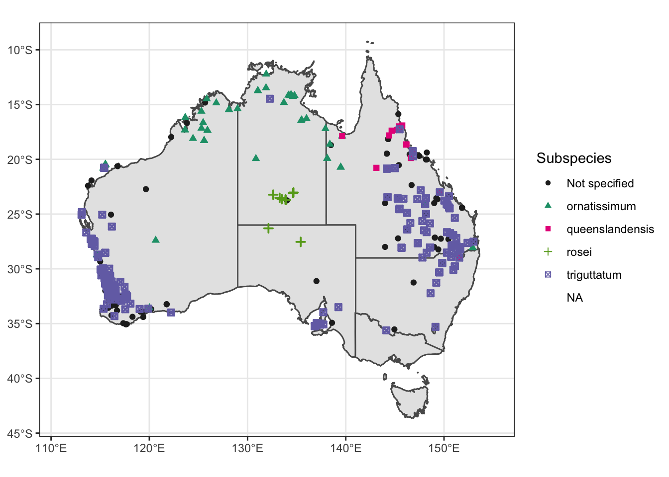
# Map without legend
Atrig2 <- Atrig1 + theme(legend.position = "none") + xlim (111, 155)
Scale for 'x' is already present. Adding another scale for 'x', which will
replace the existing scale.# Save
ggsave(
"map-atrig-subspecies1.pdf",
plot = Atrig1,
path = "output/plots",
width = 30,
height = 15,
units = "cm"
)
ggsave(
"map-atrig-subspecies2.pdf",
plot = Atrig2,
path = "output/plots",
width = 30,
height = 15,
units = "cm"
)Make simple map grouping all subspecies
Atrig3 = ggplot() +
  geom_sf(data = oz_votes) +
  geom_sf(data = oz_states,
          colour = "black",
          fill = "NA") +
  geom_point(data = obs.data.atrig,
             mapping = aes(
               x = Lon,
               y = Lat,
               color = "#7570b3",
               stroke = 1
             ))
# Customise scale
Atrig3 = Atrig3 + coord_sf() + theme_bw() + theme(
  legend.position = "none",
  axis.title.x = element_blank(),
  axis.title.y = element_blank()
)  + scale_color_manual(values = c("#7570b3")) + xlim (111,155)
Atrig3
# Remove scale
Atrig4 = Atrig3 + coord_sf() + theme_void() + theme(legend.position = "none")  + scale_color_manual(values = c("#7570b3")) +
  xlim (111,155)
Coordinate system already present. Adding new coordinate system, which will replace the existing one.Scale for 'colour' is already present. Adding another scale for 'colour',
which will replace the existing scale.Scale for 'x' is already present. Adding another scale for 'x', which will
replace the existing scale.Save map
ggsave(
  "map-atrig1.pdf",
  plot = Atrig3,
  path = "output/plots",
  width = 30,
  height = 15,
  units = "cm"
)
ggsave(
  "map-atrig2.pdf",
  plot = Atrig4,
  path = "output/plots",
  width = 30,
  height = 15,
  units = "cm"
)
Facet by Am. triguttatum subspecies map
Uee data with subspecies info and subset map
# Filter out data where subspecies is not specified
obs.data.ssp = filter(obs.data.atrig, Subspecies != "Not specified")

# make master plot
Atrig5 = ggplot() +
  geom_sf(data = oz_votes) +
  geom_sf(data = oz_states,
          colour = "black",
          fill = "NA") +
  geom_point(
    data = obs.data.ssp,
    mapping = aes(
      x = Lon,
      y = Lat,
      shape = Subspecies,
      color = Subspecies,
      stroke = 1
    )
  ) +
  coord_sf() + theme_bw() +
  theme(
    legend.position = "none",
    axis.title.x = element_blank(),
    axis.title.y = element_blank()
  ) +
  scale_color_manual(values = c("#1b9e77", "#e7298a", "#66a61e", "#7570b3")) +
  scale_shape_manual(values = c(17, 15, 3, 7)) + xlim (111, 155)
# Facet
Atrig5 = Atrig5 + facet_wrap( ~ Subspecies)
Atrig5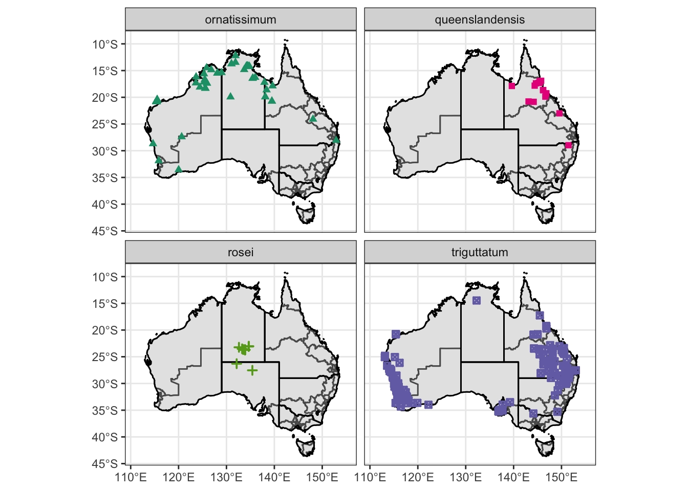
# Save
ggsave(
  "map-atrig-facet.pdf",
  plot = Atrig5,
  path = "output/plots",
  width = 30,
  height = 20,
  units = "cm"
)
Map of Ixodes holocyclus records
Load data
# raw ala records
ixhol.ala <-
  read_csv(file = "data/tick_records/ixhol/Ixhol-records-2021-02-23/records-2021-02-23.csv")
Rows: 321 Columns: 57
── Column specification ────────────────────────────────────────────────────────
Delimiter: ","
chr (40): Record ID, Catalogue Number, Taxon Concept GUID, Scientific Name ...
dbl (8): Latitude - original, Longitude - original, Latitude, Longitude, C...
lgl (8): Vernacular name, Subspecies, Coordinate Precision, IMCRA 4 Region...
date (1): Event Date - parsed
ℹ Use `spec()` to retrieve the full column specification for this data.
ℹ Specify the column types or set `show_col_types = FALSE` to quiet this message.# curated ala records - removed likely incorrect (or as a result of travel?) records from WA, SA and TAS.
obs.data.ixhol <-
read_csv(file = "data/tick_records/ixhol/Ixhol-records-2021-02-23/records-2021-02-23-curated.csv")Rows: 316 Columns: 57
── Column specification ────────────────────────────────────────────────────────
Delimiter: ","
chr (39): Record ID, Catalogue Number, Taxon Concept GUID, Scientific Name -...
dbl (10): Latitude - original, Longitude - original, Latitude, Longitude, Co...
lgl (8): Vernacular name, Subspecies, Coordinate Precision, IMCRA 4 Regions...
ℹ Use `spec()` to retrieve the full column specification for this data.
ℹ Specify the column types or set `show_col_types = FALSE` to quiet this message.Make map with state and voting outlines, overlay with all observation data
Ixhol = ggplot() +
  geom_sf(data = oz_votes) +
  geom_sf(data = oz_states,
          colour = "black",
          fill = "NA") +
  geom_point(
    data = obs.data.ixhol,
    mapping = aes(
      x = Longitude,
      y = Latitude,
      color = "#d95f02",
      stroke = 1
    )
  )
# Customise scale
Ixhol1 = Ixhol + coord_sf() + theme_bw() + theme(
  legend.position = "none",
  axis.title.x = element_blank(),
  axis.title.y = element_blank()
)  + scale_color_manual(values = c("#d95f02")) + xlim (111, 155)
Ixhol1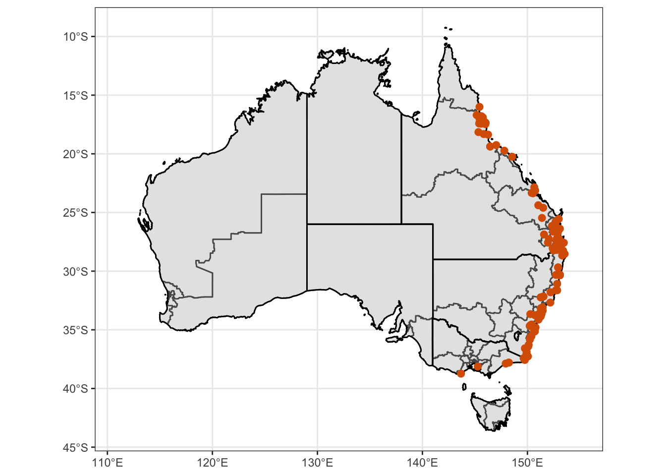
# Remove scale
Ixhol2 = Ixhol + coord_sf() + theme_void() + theme(legend.position = "none")  + scale_color_manual(values =
                                                                                                     c("#d95f02")) + xlim (111, 155)
Save maps
ggsave(
  "map-ixhol1.pdf",
  plot = Ixhol1,
  path = "output/plots",
  width = 30,
  height = 15,
  units = "cm"
)
ggsave(
  "map-ixhol2.pdf",
  plot = Ixhol2,
  path = "output/plots",
  width = 30,
  height = 15,
  units = "cm"
)
Map of Ixodes tasmani records
Load data
# curated records
obs.data.ixtas <- read_excel("data/tick_records/ixtas/curated.xlsx")
New names:
* Identifier -> Identifier...1
* Identifier -> Identifier...19Make map with state and voting outlines, overlay with all observation data
Ixtas = ggplot() +
  geom_sf(data = oz_votes) +
  geom_sf(data = oz_states,
          colour = "black",
          fill = "NA") +
  geom_point(data = obs.data.ixtas,
             mapping = aes(
               x = Lon,
               y = Lat,
               color = "#a6761d",
               stroke = 1
             ))
# Customise scale
Ixtas1 = Ixtas + coord_sf() + theme_bw() + theme(
  legend.position = "none",
  axis.title.x = element_blank(),
  axis.title.y = element_blank()
)  + scale_color_manual(values = c("#a6761d"))  + xlim (111, 155)
Ixtas1
# Remove scale
Ixtas2 = Ixtas1 + coord_sf() + theme_void() + theme(legend.position = "none")  + scale_color_manual(values =
                                                                                                      c("#a6761d")) + xlim (111, 155)
Coordinate system already present. Adding new coordinate system, which will replace the existing one.Scale for 'colour' is already present. Adding another scale for 'colour',
which will replace the existing scale.Scale for 'x' is already present. Adding another scale for 'x', which will
replace the existing scale.Save maps
ggsave(
  "map-ixtas1.pdf",
  plot = Ixtas1,
  path = "output/plots",
  width = 30,
  height = 15,
  units = "cm"
)
ggsave(
  "map-ixtas2.pdf",
  plot = Ixtas2,
  path = "output/plots",
  width = 30,
  height = 15,
  units = "cm"
)
Combined map
Make combine map of Am. trig, Ix. hol and Ix. tas.
Using Am. triguttatum subspecies maps
figure1 <- ggarrange(
  Atrig2,
  Ixhol1,
  Ixtas1,
  labels = c("A", "B", "C"),
  ncol = 2,
  nrow = 2
)
ggsave(
  "combined-map1.pdf",
  plot = figure1,
  path = "output/plots",
  width = 30,
  height = 15,
  units = "cm"
)
figure1

figure2 <- ggarrange(Atrig2,
                     Ixhol1,
                     Ixtas1,
                     labels = c("A", "B", "C"),
                     nrow = 3)
ggsave(
  "combined-map2.pdf",
  plot = figure2,
  path = "output/plots",
  width = 30,
  height = 15,
  units = "cm"
)
figure2

figure3 <- ggarrange(Atrig2,
                     Ixhol1,
                     Ixtas1,
                     labels = c("A", "B", "C"),
                     ncol = 3)
ggsave(
  "combined-map3.pdf",
  plot = figure3,
  path = "output/plots",
  width = 30,
  height = 15,
  units = "cm"
)
figure3
gp <- ggarrange(
Atrig2,
# First row with line plot
# Second row with box and dot plots
ggarrange(Ixhol1, Ixtas1, ncol = 2, labels = c("B", "C")),
nrow = 2,
labels = "A" # Label of the line plot
)
gp
ggsave(
"combined-map4.pdf",
plot = gp,
path = "output/plots",
width = 30,
height = 15,
units = "cm"
)Using Am. triguttatum combine maps
figure1 <- ggarrange(
  Atrig3,
  Ixhol1,
  Ixtas1,
  labels = c("A", "B", "C"),
  ncol = 2,
  nrow = 2
)
ggsave(
  "combined-map5.pdf",
  plot = figure1,
  path = "output/plots",
  width = 30,
  height = 15,
  units = "cm"
)
figure1

figure2 <- ggarrange(Atrig3,
                     Ixhol1,
                     Ixtas1,
                     labels = c("A", "B", "C"),
                     nrow = 3)
ggsave(
  "combined-map6.pdf",
  plot = figure2,
  path = "output/plots",
  width = 30,
  height = 15,
  units = "cm"
)
figure2

figure3 <- ggarrange(Atrig3,
                     Ixhol1,
                     Ixtas1,
                     labels = c("A", "B", "C"),
                     ncol = 3)
ggsave(
  "combined-map7.pdf",
  plot = figure3,
  path = "output/plots",
  width = 30,
  height = 15,
  units = "cm"
)
figure3
gp <- ggarrange(
Atrig3,
# First row with line plot
# Second row with box and dot plots
ggarrange(Ixhol1, Ixtas1, ncol = 2, labels = c("B", "C")),
nrow = 2,
labels = "A" # Label of the line plot
)
gp
ggsave(
"combined-map8.pdf",
plot = gp,
path = "output/plots",
width = 30,
height = 15,
units = "cm"
)All records of Australian ticks
Curated data
First set of plots contains occurance data from curated plots Load data which contains combined records from ANIC, WAM, Living Atlas Australia and publications.
raw_records <- read_csv("data/tick_records/comb_tick_records.csv")Rows: 8446 Columns: 23
── Column specification ────────────────────────────────────────────────────────
Delimiter: ","
chr (21): source, accession, COUNTRY, STATE, LOCALITY 1, LOCALITY 2, COLLECT...
dbl (2): LATITUDE, LONGITUDE
ℹ Use `spec()` to retrieve the full column specification for this data.
ℹ Specify the column types or set `show_col_types = FALSE` to quiet this message.head(raw_records)# A tibble: 6 × 23
source accession COUNTRY STATE `LOCALITY 1` `LOCALITY 2` LATITUDE LONGITUDE
<chr> <chr> <chr> <chr> <chr> <chr> <dbl> <dbl>
1 ANIC 48 000 001 <NA> WA Mileura Stati… 15 miles SE -26.5 118.
2 ANIC 48 000 002 <NA> <NA> <NA> <NA> NA NA
3 ANIC 48 000 003 Iraq <NA> <NA> <NA> NA NA
4 ANIC 48 000 004 <NA> <NA> <NA> <NA> NA NA
5 ANIC 48 000 005 <NA> NSW Glencoe near Graves… -29.6 150.
6 ANIC 48 000 006 <NA> SA Clare 10 miles N -33.7 139.
# … with 15 more variables: COLLECTOR <chr>, DATE <chr>, FAMILY <chr>,
# GENUS <chr>, SPECIES <chr>, SUBSPECIES <chr>, STAGE <chr>,
# IDENTIFIED <chr>, `SPECIMEN STATUS` <chr>, NOTES <chr>, TYPE <chr>,
# `HOST COMMON NAME` <chr>, `HOST GENUS` <chr>, `HOST SPECIES` <chr>,
# HABITAT <chr>Clean up data
Correct states
clean_records <- raw_records

unique(clean_records$STATE)
[1] "WA" NA "NSW"
[4] "SA" "QLD" "ACT"
[7] "VIC" "NT" "QLD ?"
[10] "TAS" "Coral Sea Territory" "California"
[13] "Hidalgo" "Morelos" "Missouri"
[16] "Virginia" "?" "Perak"
[19] "Vera Cruz" "Tabasco" "Nayarit"
[22] "Texas" "Tennessee" "Coahuila"
[25] "Florida" "Papua" "Vic"
[28] "Nigata Prefecture" "NSW or SA" "Niigata Prefecture"
[31] "Dhofar Province" "Pahang" "NSW/QLD"
[34] "Gujarat" "Queretaro" "Sumatra"
[37] "Christmas Island" "Nevada" "Veracruz"
[40] "W.A." "N.S.W." "N.T."
[43] "Qld" "S.A." "West Timor"
[46] "Maluku Province" "Tas." "Vic."
[49] "Washington" clean_records$STATE[clean_records$STATE == "W.A."] <- "WA"
clean_records$STATE[clean_records$STATE == "QLD ?"] <- "QLD"
clean_records$STATE[clean_records$STATE == "NSW/QLD"] <- ""
clean_records$STATE[clean_records$STATE == "NSW or SA"] <- ""
clean_records$STATE[clean_records$STATE == "N.S.W."] <- "NSW"
clean_records$STATE[clean_records$STATE == "Vic"] <- "VIC"
clean_records$STATE[clean_records$STATE == "N.T."] <- "NT"
clean_records$STATE[clean_records$STATE == "Qld"] <- "QLD"
clean_records$STATE[clean_records$STATE == "S.A."] <- "SA"
clean_records$STATE[clean_records$STATE == "Tas."] <- "TAS"
clean_records$STATE[clean_records$STATE == "Vic."] <- "VIC"Update and correct taxonomy of tick genus and species names
clean_records$GENUS[clean_records$GENUS == "Aponomma"] <-
  "Bothriocroton"
clean_records$SPECIES[clean_records$SPECIES == "sanguinensis"] <-
  "sanguineus"

clean_records$genusspecies <-
  paste(clean_records$GENUS, clean_records$SPECIES)
unique(clean_records$genusspecies)
[1] "Argas falco" "Argas hermanni"
[3] "Argas lagenoplastis" "Argas nullarborensis"
[5] "Argas persicus" "Argas robertsi"
[7] "Argas vespertilionis" "Argas NA"
[9] "Carios australiensis" "Carios capensis"
[11] "Carios daviesi" "Carios dewae"
[13] "Carios macrodermae" "Ornithodoros batuensis"
[15] "Ornithodoros coriaceus" "Ornithodoros faini"
[17] "Ornithodoros gurneyi" "Ornithodoros macmillani"
[19] "Ornithodoros moubata" "Ornithodoros papuensis"
[21] "Ornithodoros periformis ?" "Ornithodoros salahi"
[23] "Ornithodoros savignyi" "Ornithodoros NA"
[25] "Otobius megnini" "Amblyomma albolimbatum"
[27] "Amblyomma triguttatum" "Amblyomma americanum"
[29] "Amblyomma australiense" "Amblyomma breviscutatum"
[31] "Amblyomma calabyi" "Amblyomma cayennense"
[33] "Amblyomma cohaerens" "Amblyomma cuneatum"
[35] "Amblyomma dissimile" "Amblyomma echidnae"
[37] "Amblyomma fimbriatum" "Amblyomma flavomaculatum"
[39] "Amblyomma geayi" "Amblyomma gemma"
[41] "Amblyomma hebraeum" "Amblyomma helvolum"
[43] "Amblyomma imitator" "Amblyomma javanense"
[45] "Amblyomma lepidum" "Amblyomma limbatum"
[47] "Amblyomma loculosum" "Amblyomma maculatum"
[49] "Amblyomma marmoreum" "Amblyomma moreliae"
[51] "Amblyomma moyi" "Amblyomma papuanum"
[53] "Amblyomma pictum" "Amblyomma postoculatum"
[55] "Amblyomma thalloni" "Amblyomma trimaculatum"
[57] "Amblyomma variegatum" "Amblyomma NA"
[59] "Anocentor nitens" "Bothriocroton elaphensis"
[61] "Bothriocroton exornatum" "Bothriocroton lucasi"
[63] "Bothriocroton auruginans" "Bothriocroton concolor"
[65] "Bothriocroton hydrosauri" "Bothriocroton tachyglossi"
[67] "Bothriocroton undatum" "Dermacentor albipictus"
[69] "Dermacentor andersoni" "Dermacentor auratus"
[71] "Dermacentor nigrolineatus" "Dermacentor occidentalis"
[73] "Dermacentor parumapertus" "Dermacentor variabilis"
[75] "Haemaphysalis bancrofti" "Haemaphysalis bremneri"
[77] "Haemaphysalis campanulata" "Haemaphysalis cornigera"
[79] "Haemaphysalis doenitzi" "Haemaphysalis flava"
[81] "Haemaphysalis humerosa" "Haemaphysalis hystricis"
[83] "Haemaphysalis japonica" "Haemaphysalis lagostrophi"
[85] "Haemaphysalis leachi" "Haemaphysalis longicornis"
[87] "Haemaphysalis bispinosa" "Haemaphysalis neumanni"
[89] "Haemaphysalis novaeguineae" "Haemaphysalis papuana"
[91] "Haemaphysalis petrogalis" "Haemaphysalis ratti"
[93] "Haemaphysalis sulcata" "Haemaphysalis wellingtoni"
[95] "Haemaphysalis NA" "Hyalomma aegyptium"
[97] "Hyalomma albiparmatum" "Hyalomma anatolicum"
[99] "Hyalomma asiaticum" "Hyalomma dentritum"
[101] "Hyalomma dromedarii" "Hyalomma impeltatum"
[103] "Hyalomma marginatum" "Hyalomma rufipes"
[105] "Hyalomma savignyi" "Hyalomma schulzei"
[107] "Hyalomma truncatum" "Hyalomma NA"
[109] "Ixodes antechini" "Ixodes auritulus"
[111] "Ixodes australiensis" "Ixodes canisuga"
[113] "Ixodes confusus" "Ixodes cordifer"
[115] "Ixodes cornuatus" "Ixodes holocyclus"
[117] "Ixodes eichhorni" "Ixodes eudyptidis"
[119] "Ixodes laridis" "Ixodes fecialis"
[121] "Ixodes heathi" "Ixodes granulatus"
[123] "Ixodes hexagonus" "Ixodes hirsti"
[125] "Ixodes hydromyidis" "Ixodes kerguelenensis"
[127] "Ixodes kohlsi" "Ixodes kopsteini"
[129] "Ixodes luxuriosus" "Ixodes myrmecobii"
[131] "Ixodes ornithorhynchi" "Ixodes ovatus"
[133] "Ixodes pilosus" "Ixodes ricinus"
[135] "Ixodes rubicundus" "Ixodes scapularis"
[137] "Ixodes simplex" "Ixodes tasmani"
[139] "NA NA" "Ixodes trichosuri"
[141] "Ixodes uriae" "Ixodes vestitus"
[143] "Ixodes victoriensis" "Ixodes NA"
[145] "Margaropus winthemi" "Nosomma monstrosum"
[147] "Rhipicephalus annulatus" "Rhipicephalus appendiculatus"
[149] "Rhipicephalus bursa" "Rhipicephalus capensis"
[151] "Rhipicephalus compositus" "Rhipicephalus decoloratus"
[153] "Rhipicephalus evertsi" "Rhipicephalus kohlsi"
[155] "Rhipicephalus haemaphysaloides" "Rhipicephalus longus"
[157] "Rhipicephalus microplus" "Rhipicephalus nymphae"
[159] "Rhipicephalus pravus" "Rhipicephalus pulchellus"
[161] "Rhipicephalus rubicundus" "Rhipicephalus rufipes"
[163] "Rhipicephalus sanguineus" "Rhipicephalus secundus"
[165] "Rhipicephalus simus" "Rhipicephalus supertritus"
[167] "Rhipicephalus zambeziensis" "Rhipicephalus NA"
[169] "Bothriocroton NA" "Rhipicephalus australis"
[171] "Argas/Carios NA" "Dermacentor vaiabilis"
[173] "Ixodes ornithoryhnchi" "Amblyomma sp."
[175] "Haemaphysalis sp." "Amblyomma glauerti"
[177] "Amblyomma soembawensis" "Bothriocroton sp."
[179] "Bothriocroton glebopalma" "Dermacentor NA"
[181] "Ixodes sp." "Ixodes woyliei"
[183] "Amblyomma macropi" "Ixodes barkeri"
[185] "Amblyomma viikirri" "Argas lowryae" Filter records
comb_records_filt <- clean_records %>%
  filter(!is.na(LATITUDE)) %>%
  filter(!is.na(SPECIES)) %>%
  filter(!SPECIES == "sp.")
Merge with previous records
Merge full records with curated records for Am. triguttatum, Ix. holocyclus and Ix. tasmani.
df1 <-
  comb_records_filt %>% select(LATITUDE, LONGITUDE, genusspecies)

df2 <- obs.data.atrig
df2$genusspecies <- paste(df2$Tick_genus, df2$Tick_species)
df2 <- df2 %>% select(Lat, Lon, genusspecies)
df2 <- rename(df2,
              LATITUDE = Lat,
              LONGITUDE = Lon)

df3 <- obs.data.ixhol %>% select(Latitude, Longitude, Species)
df3 <- rename(df3,
              LATITUDE = Latitude,
              LONGITUDE = Longitude,
              genusspecies = Species)

df4 <- obs.data.ixtas
df4$genusspecies <- paste(df4$Tick_genus, df4$Tick_species)
df4 <- df4 %>% select(Lat, Lon, genusspecies)
df4 <- rename(df4,
              LATITUDE = Lat,
              LONGITUDE = Lon)

tick.obs.data <- rbind(df1, df2, df3, df4)
Final filter of records - also filtering single record of Argas vespertilionis in WAM database - I think given single record this is most likely an incorrect identification.
# # remove overseas species
overseas_ticks <-
  c(
    "Amblyomma soembawensis",
    "Dermacentor variabilis",
    "Rhipicephalus appendiculatus",
    "Rhipicephalus microplus",
    "Margaropus winthemi",
    "Argas vespertilionis",
    "NA NA"
  )

tick.obs.data <- tick.obs.data %>%
  filter(!is.na(LATITUDE)) %>%
  filter(!genusspecies %in% overseas_ticks)
Plot
Make combined plot of all tick species recorded in Australia.
oz_states <- ozmaps::ozmap_states

oz_states <-
  ozmaps::ozmap_states %>% filter(NAME != "Other Territories")
oz_votes <- rmapshaper::ms_simplify(ozmaps::abs_ced)
Set order for the legend by tick genera.
levels(tick.obs.data$genusspecies)NULLtick.obs.data$genusspecies <- as.factor(tick.obs.data$genusspecies)
levels(tick.obs.data$genusspecies) [1] "Amblyomma albolimbatum" "Amblyomma australiense"
[3] "Amblyomma breviscutatum" "Amblyomma calabyi"
[5] "Amblyomma echidnae" "Amblyomma fimbriatum"
[7] "Amblyomma glauerti" "Amblyomma limbatum"
[9] "Amblyomma loculosum" "Amblyomma macropi"
[11] "Amblyomma moreliae" "Amblyomma moyi"
[13] "Amblyomma papuanum" "Amblyomma postoculatum"
[15] "Amblyomma triguttatum" "Amblyomma trimaculatum"
[17] "Amblyomma viikirri" "Argas falco"
[19] "Argas lagenoplastis" "Argas lowryae"
[21] "Argas nullarborensis" "Argas persicus"
[23] "Argas robertsi" "Bothriocroton auruginans"
[25] "Bothriocroton concolor" "Bothriocroton glebopalma"
[27] "Bothriocroton hydrosauri" "Bothriocroton tachyglossi"
[29] "Bothriocroton undatum" "Carios australiensis"
[31] "Carios capensis" "Carios daviesi"
[33] "Carios dewae" "Carios macrodermae"
[35] "Haemaphysalis bancrofti" "Haemaphysalis bremneri"
[37] "Haemaphysalis doenitzi" "Haemaphysalis humerosa"
[39] "Haemaphysalis lagostrophi" "Haemaphysalis longicornis"
[41] "Haemaphysalis novaeguineae" "Haemaphysalis petrogalis"
[43] "Haemaphysalis ratti" "Ixodes antechini"
[45] "Ixodes auritulus" "Ixodes australiensis"
[47] "Ixodes barkeri" "Ixodes confusus"
[49] "Ixodes cordifer" "Ixodes cornuatus"
[51] "Ixodes eudyptidis" "Ixodes fecialis"
[53] "Ixodes heathi" "Ixodes hirsti"
[55] "Ixodes holocyclus" "Ixodes hydromyidis"
[57] "Ixodes kerguelenensis" "Ixodes kohlsi"
[59] "Ixodes kopsteini" "Ixodes laridis"
[61] "Ixodes myrmecobii" "Ixodes ornithorhynchi"
[63] "Ixodes simplex" "Ixodes tasmani"
[65] "Ixodes trichosuri" "Ixodes uriae"
[67] "Ixodes vestitus" "Ixodes victoriensis"
[69] "Ixodes woyliei" "Ornithodoros gurneyi"
[71] "Ornithodoros macmillani" "Otobius megnini"
[73] "Rhipicephalus australis" "Rhipicephalus sanguineus" tick.obs.data$genusspecies <-
factor(
tick.obs.data$genusspecies,
levels = c(
"Amblyomma albolimbatum",
"Amblyomma australiense",
"Amblyomma breviscutatum",
"Amblyomma calabyi",
"Amblyomma echidnae",
"Amblyomma fimbriatum",
"Amblyomma glauerti",
"Amblyomma limbatum",
"Amblyomma loculosum",
"Amblyomma macropi",
"Amblyomma moreliae",
"Amblyomma moyi",
"Amblyomma papuanum",
"Amblyomma postoculatum",
"Amblyomma triguttatum",
"Amblyomma trimaculatum",
"Amblyomma viikirri",
"Bothriocroton auruginans",
"Bothriocroton concolor",
"Bothriocroton glebopalma",
"Bothriocroton hydrosauri",
"Bothriocroton tachyglossi",
"Bothriocroton undatum",
"Haemaphysalis bancrofti",
"Haemaphysalis bremneri",
"Haemaphysalis doenitzi",
"Haemaphysalis humerosa",
"Haemaphysalis lagostrophi",
"Haemaphysalis longicornis",
"Haemaphysalis novaeguineae",
"Haemaphysalis petrogalis",
"Haemaphysalis ratti",
"Ixodes antechini",
"Ixodes auritulus",
"Ixodes australiensis",
"Ixodes barkeri",
"Ixodes confusus",
"Ixodes cordifer",
"Ixodes cornuatus",
"Ixodes eudyptidis",
"Ixodes fecialis",
"Ixodes heathi",
"Ixodes hirsti",
"Ixodes holocyclus",
"Ixodes hydromyidis",
"Ixodes kerguelenensis",
"Ixodes kohlsi",
"Ixodes kopsteini",
"Ixodes laridis",
"Ixodes myrmecobii",
"Ixodes ornithorhynchi",
"Ixodes simplex",
"Ixodes tasmani",
"Ixodes trichosuri",
"Ixodes uriae",
"Ixodes vestitus",
"Ixodes victoriensis",
"Ixodes woyliei",
"Rhipicephalus australis",
"Rhipicephalus sanguineus",
"Argas falco",
"Argas lagenoplastis",
"Argas lowryae",
"Argas nullarborensis",
"Argas persicus",
"Argas robertsi",
"Carios australiensis",
"Carios capensis",
"Carios daviesi",
"Carios dewae",
"Carios macrodermae",
"Ornithodoros gurneyi",
"Ornithodoros macmillani",
"Otobius megnini"
)
)p <- ggplot() +
geom_sf(data = oz_votes) +
geom_sf(data = oz_states, colour = "black", fill = "NA") +
geom_point(
data = tick.obs.data,
mapping = aes(
x = LONGITUDE,
y = LATITUDE,
color = genusspecies
)) +
labs(
x = "Longitude",
y = "Latitude",
colour = "Tick species",
title = "Ticks of Australia"
)
p1 <-
p + xlim (112, 154) + ylim (-45, -8) + theme_classic() + scale_color_viridis(discrete =
TRUE)
ggplotly(p1)p1.plotly <- plotly::ggplotly(p1)
htmlwidgets::saveWidget(p1.plotly, "output/plots/map-all-curated.html")Data behind the map
Occurrence of data of Australian ticks.
All Living Atlas Australia records.
Search of Living Atlas Australia using taxonomic classification “Ixodida” (Order level).
obs.data.ala <-
  read_csv("data/tick_records/IXODIDA-records-2022-02-27/records-2022-02-27.csv")
New names:
* images -> images...2
* locality -> locality...75
* locality -> locality...76
* verbatimElevation -> verbatimElevation...80
* verbatimElevation -> verbatimElevation...81
* ...Rows: 7149 Columns: 167
── Column specification ────────────────────────────────────────────────────────
Delimiter: ","
chr (85): dataResourceUid, images...2, raw_recordedBy, dcterms:language, dc...
dbl (13): individualCount, year, month, day, minimumElevationInMeters, deci...
lgl (67): dcterms:accessRights, informationWithheld, dataGeneralizations, o...
dttm (2): dcterms:modified, eventDate
ℹ Use `spec()` to retrieve the full column specification for this data.
ℹ Specify the column types or set `show_col_types = FALSE` to quiet this message.# Filter out data without species and no coordinates
obs.data.ala <- obs.data.ala %>%
filter(!is.na(species)) %>%
filter(!is.na(decimalLatitude))obs.data.ala$species[obs.data.ala$species=="Argas dewae"]<-"Carios dewae"
obs.data.ala$species[obs.data.ala$species=="Argas macrodermae"]<-"Carios macrodermae"Prepare base map
oz_states <- ozmaps::ozmap_states

oz_states <-
  ozmaps::ozmap_states %>% filter(NAME != "Other Territories")
oz_votes <- rmapshaper::ms_simplify(ozmaps::abs_ced)
Set order for the legend by tick genera.
levels(obs.data.ala$species)NULLobs.data.ala$species <- as.factor(obs.data.ala$species)
levels(obs.data.ala$species) [1] "Amblyomma albolimbatum" "Amblyomma australiense"
[3] "Amblyomma calabyi" "Amblyomma echidnae"
[5] "Amblyomma fimbriatum" "Amblyomma flavomaculatum"
[7] "Amblyomma glauerti" "Amblyomma limbatum"
[9] "Amblyomma loculosum" "Amblyomma macropi"
[11] "Amblyomma moreliae" "Amblyomma moyi"
[13] "Amblyomma postoculatum" "Amblyomma triguttatum"
[15] "Amblyomma trimaculatum" "Amblyomma vikirri"
[17] "Argas lagenoplastis" "Argas persicus"
[19] "Argas robertsi" "Bothriocroton auruginans"
[21] "Bothriocroton concolor" "Bothriocroton glebopalma"
[23] "Bothriocroton hydrosauri" "Bothriocroton tachyglossi"
[25] "Bothriocroton undatum" "Carios dewae"
[27] "Carios macrodermae" "Haemaphysalis bancrofti"
[29] "Haemaphysalis humerosa" "Haemaphysalis lagostrophi"
[31] "Haemaphysalis longicornis" "Haemaphysalis petrogalis"
[33] "Haemaphysalis ratti" "Ixodes antechini"
[35] "Ixodes auritulus" "Ixodes australiensis"
[37] "Ixodes cordifer" "Ixodes cornuatus"
[39] "Ixodes eudyptidis" "Ixodes fecialis"
[41] "Ixodes heathi" "Ixodes hirsti"
[43] "Ixodes holocyclus" "Ixodes hydromyidis"
[45] "Ixodes kerguelenensis" "Ixodes kohlsi"
[47] "Ixodes myrmecobii" "Ixodes ornithorhynchi"
[49] "Ixodes tasmani" "Ixodes trichosuri"
[51] "Ixodes uriae" "Ixodes victoriensis"
[53] "Ixodes woyliei" "Ornithodoros gurneyi"
[55] "Ornithodoros macmillani" "Rhipicephalus australis"
[57] "Rhipicephalus sanguineus" obs.data.ala$species <- factor(
obs.data.ala$species,
levels = c(
"Amblyomma albolimbatum",
"Amblyomma australiense",
"Amblyomma calabyi",
"Amblyomma echidnae",
"Amblyomma fimbriatum",
"Amblyomma flavomaculatum",
"Amblyomma glauerti",
"Amblyomma limbatum",
"Amblyomma loculosum",
"Amblyomma macropi",
"Amblyomma moreliae",
"Amblyomma moyi",
"Amblyomma postoculatum",
"Amblyomma triguttatum",
"Amblyomma trimaculatum",
"Amblyomma viikirri",
"Bothriocroton auruginans",
"Bothriocroton concolor",
"Bothriocroton glebopalma",
"Bothriocroton hydrosauri",
"Bothriocroton tachyglossi",
"Bothriocroton undatum",
"Haemaphysalis bancrofti",
"Haemaphysalis humerosa",
"Haemaphysalis lagostrophi",
"Haemaphysalis longicornis",
"Haemaphysalis petrogalis",
"Haemaphysalis ratti",
"Ixodes antechini",
"Ixodes auritulus",
"Ixodes australiensis",
"Ixodes cordifer",
"Ixodes cornuatus",
"Ixodes eudyptidis",
"Ixodes fecialis",
"Ixodes heathi",
"Ixodes hirsti",
"Ixodes holocyclus",
"Ixodes hydromyidis",
"Ixodes kerguelenensis",
"Ixodes kohlsi",
"Ixodes myrmecobii",
"Ixodes ornithorhynchi",
"Ixodes tasmani",
"Ixodes trichosuri",
"Ixodes uriae",
"Ixodes victoriensis",
"Ixodes woyliei",
"Rhipicephalus australis",
"Rhipicephalus sanguineus",
"Argas lagenoplastis",
"Argas persicus",
"Argas robertsi",
"Carios dewae",
"Carios macrodermae",
"Ornithodoros gurneyi",
"Ornithodoros macmillani"
)
)p <- ggplot() +
geom_sf(data = oz_votes) +
geom_sf(data = oz_states, colour = "black", fill = "NA") +
geom_point(
data = obs.data.ala,
mapping = aes(
x = decimalLongitude,
y = decimalLatitude,
color = species
)) +
labs(
x = "Longitude",
y = "Latitude",
colour = "Tick species",
title = "Ticks of Australia - Living Atlas Australia Records"
)
p1 <- p + xlim (112,154) + ylim (-45,-8) + theme_classic() + scale_color_viridis(discrete=TRUE)
ggplotly(p1)p1.plotly <- plotly::ggplotly(p1)
htmlwidgets::saveWidget(p1.plotly, "output/plots/map-all-ala.html")
sessionInfo()R version 4.1.2 (2021-11-01)
Platform: x86_64-apple-darwin17.0 (64-bit)
Running under: macOS Catalina 10.15.7
Matrix products: default
BLAS: /Library/Frameworks/R.framework/Versions/4.1/Resources/lib/libRblas.0.dylib
LAPACK: /Library/Frameworks/R.framework/Versions/4.1/Resources/lib/libRlapack.dylib
locale:
[1] en_AU.UTF-8/en_AU.UTF-8/en_AU.UTF-8/C/en_AU.UTF-8/en_AU.UTF-8
attached base packages:
[1] stats graphics grDevices utils datasets methods base
other attached packages:
[1] readxl_1.3.1 forcats_0.5.1 stringr_1.4.0 dplyr_1.0.8
[5] purrr_0.3.4 readr_2.1.2 tidyr_1.2.0 tibble_3.1.6
[9] tidyverse_1.3.1 plotly_4.10.0 viridis_0.6.2 viridisLite_0.4.0
[13] ggpubr_0.4.0 ggplot2_3.3.5 rmapshaper_0.4.5 raster_3.5-15
[17] rgdal_1.5-28 sp_1.4-6 sf_1.0-6 ozmaps_0.4.5
[21] workflowr_1.7.0
loaded via a namespace (and not attached):
[1] colorspace_2.0-3 ggsignif_0.6.3 ellipsis_0.3.2
[4] class_7.3-20 rprojroot_2.0.2 fs_1.5.2
[7] httpcode_0.3.0 rstudioapi_0.13 proxy_0.4-26
[10] farver_2.1.0 bit64_4.0.5 fansi_1.0.2
[13] lubridate_1.8.0 xml2_1.3.3 codetools_0.2-18
[16] knitr_1.37 geojsonlint_0.4.0 jsonlite_1.8.0
[19] broom_0.7.12 dbplyr_2.1.1 rgeos_0.5-9
[22] compiler_4.1.2 httr_1.4.2 backports_1.4.1
[25] assertthat_0.2.1 fastmap_1.1.0 lazyeval_0.2.2
[28] cli_3.2.0 s2_1.0.7 later_1.3.0
[31] htmltools_0.5.2 tools_4.1.2 gtable_0.3.0
[34] glue_1.6.2 geojson_0.3.4 wk_0.6.0
[37] V8_4.1.0 Rcpp_1.0.8 carData_3.0-5
[40] cellranger_1.1.0 oz_1.0-21 jquerylib_0.1.4
[43] vctrs_0.3.8 crul_1.2.0 crosstalk_1.2.0
[46] xfun_0.29 ps_1.6.0 rvest_1.0.2
[49] lifecycle_1.0.1 rstatix_0.7.0 terra_1.5-21
[52] jqr_1.2.2 getPass_0.2-2 scales_1.1.1
[55] vroom_1.5.7 hms_1.1.1 promises_1.2.0.1
[58] parallel_4.1.2 yaml_2.3.5 curl_4.3.2
[61] gridExtra_2.3 sass_0.4.0 stringi_1.7.6
[64] jsonvalidate_1.3.2 highr_0.9 maptools_1.1-2
[67] e1071_1.7-9 rlang_1.0.1 pkgconfig_2.0.3
[70] evaluate_0.15 lattice_0.20-45 htmlwidgets_1.5.4
[73] bit_4.0.4 processx_3.5.2 tidyselect_1.1.2
[76] magrittr_2.0.2 geojsonsf_2.0.1 R6_2.5.1
[79] geojsonio_0.9.4 generics_0.1.2 DBI_1.1.2
[82] foreign_0.8-82 pillar_1.7.0 haven_2.4.3
[85] whisker_0.4 withr_2.4.3 units_0.8-0
[88] abind_1.4-5 modelr_0.1.8 crayon_1.5.0
[91] car_3.0-12 KernSmooth_2.23-20 utf8_1.2.2
[94] tzdb_0.2.0 rmarkdown_2.11.22 grid_4.1.2
[97] data.table_1.14.2 callr_3.7.0 git2r_0.29.0
[100] reprex_2.0.1 digest_0.6.29 classInt_0.4-3
[103] httpuv_1.6.5 munsell_0.5.0 bslib_0.3.1